Introduction

Hydroacoustics – using sound to ‘see’ in the ocean – has become central to evidence-based ocean management and mapping marine life. Marine scientists rely on echosounders to estimate abundance indices for assessments of biomass, while regulators and developers use the same tools to assess ecological impacts around offshore energy sites.

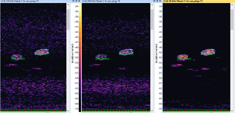
Hull‑mounted echosounders used in active acoustic surveys work by emitting pulses of sound and measuring the strength of the returning echoes. These backscatter signals contain information about the distribution and abundance of marine organisms throughout the water column.

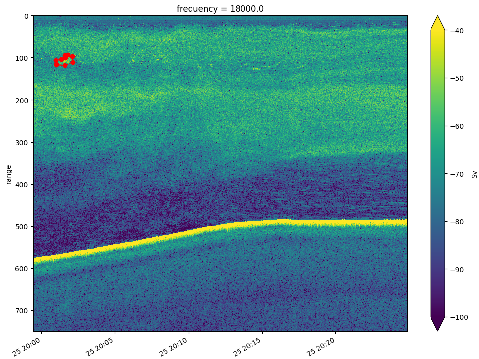
This information is plotted as what we call echograms – two‑dimensional visualisations of the volume backscattering strength (Sv) over time and depth and are used by researchers to identify pelagic fish schools, scattering layers and the seabed.

In this article we present a comprehensive implementation of an Edge‑to‑Cloud ML-based pipeline in which we trained and deployed a model for semantic segmentation of echograms. The model was packaged and deployed as an IoT Edge module, using the framework we're developing at OceanStream, then tested in a simulated live environment to predict fish schools in multifrequency echosounder data.

This work was presented at the 2025 ICES WGFAST workshop, which was held at MFRI in Iceland between 8-13 of April.

Active Acoustics Primer

Active acoustics rely on emitting sound pulses and interpreting the echoes from the water column to infer the presence and density of organisms. Water‑column sonar data captured by active acoustic instruments, such as echosounders, contain scattering information from the near‑surface to the seafloor, allowing marine scientists to assess the spatial distribution of plankton, fish and other marine life.

These data is combined with CTD (conductivity‑temperature‑depth) profiles, trawl catches and camera footage to identify the species responsible for specific acoustic signatures and then produce abundance estimates and develop ecosystem models.

In our experiment, the target species was Atlantic herring (Clupea harengus) – a cornerstone of the Northwest Atlantic ecosystem which play a dual role as an ecologically important forage species and an economically valuable commercial fishing resource. The Atlantic States Marine Fisheries Commission notes that herring serve as a key forage fish for marine mammals, seabirds and a wide range of predatory fish from Labrador to Virginia. Their schooling behaviour makes them an important prey resource for migrating whales and dolphins.

In recent years herring stocks have declined however, which resulted in tighter management measures that underscores the need for accurate population monitoring, and acoustic methods are well suited to estimate their abundance and spatial distribution due to the large, dynamic schools which these pelagic fish form.

Data Acquisition and Preparation

We used data collected by the NEFSC 2019 Fall Bottom Trawl Survey – a fisheries independent, multi-species survey conducted by the NOAA Northeast Fisheries Science Center. The survey is comprised of two bottom trawl cruises each year, one in the spring and one in the autumn, that provide the primary scientific data for fisheries assessments in the U.S. mid-Atlantic and New England regions.

The data was collected by the NOAA Ship Henry B. Bigelow during both daytime and nighttime (Politis et al. 2014). Acoustic data consisted of multifrequency Simrad EK60 echosounder narrowband (i.e., continuous wave, CW) data at 18, 38, 70, 120, and 200 kHz (Zhang et al 2024).

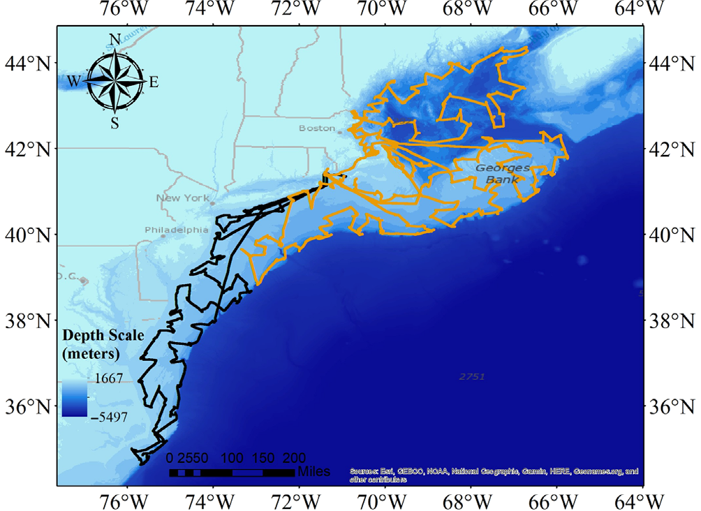
The raw data is available in a public-access S3 bucket on AWS here, part of the NOAA NCEI archive. We selected 18 days of observations.

Manual Annotations

The acoustic data were accompanied by region annotations of fish schools produced in the Echoview software, the leading desktop suite for hydroacoustic data analysis, and exported to EVR files – an open format generated by the echoregions library. Experts at NEFSC labelled regions belonging to four classes of annotations: positive target “Atlantic herring school”, and negative non-target “Clupeid school”, “Krill” and “Noise region” (Zhang et al 2024).

For the purposes of this experiment all fish classes were collapsed to two binary classes (Fish vs Background) for segmentation. After filtering bad data (based on vessel logs and EVR flags) and removing empty pings, we segmented each day into image “chips” and kept only those with non‑empty masks, yielding 362 2‑D segments (10% test split). Augmentations included random square crops, horizontal flips, resize to 512×512, and ImageNet normalisation.

Data preprocessing and augmentation

We convert raw EK60 files into cloud‑optimised arrays using echopype, which implements the SONAR‑netCDF4 convention and writes Zarr for chunked, lazy access – ideal for distributed training and analysis. Preprocessing transforms the raw acoustic data into images suitable for convolutional networks.

Each dataset was cut into segments of the size max_depth * 1.5. Only those segments were kept, for which the mask derived from the EVR file was not empty. In total, 362 segments were generated. These were the images used for training and testing the model.

Each segment is min–max normalised independently to account for varying signal intensities, and missing values are imputed with small negative numbers. The first three frequency channels are mapped to the red, green and blue channels of an RGB image. 

To augment the limited data, 50 % of the images are horizontally flipped, and all are resized to a resolution of 512 × 512 pixels. When using ImageNet‑pretrained encoders, the images are normalised with the mean and standard deviation of the ImageNet dataset.

Model Architecture and Training

The segmentation task is formulated as a pixel‑wise binary classification: each pixel in the echogram is assigned to either the Fish class or the Background. In this study several encoder–decoder networks from the Pytorch library were benchmarked.

Three convolutional architectures were tested: 

1. U‑Net
2. DeepLabV3+
3. Feature-Pyramid-Network (FPN)

U‑Net, originally developed for biomedical imaging, uses symmetrical encoder and decoder paths with skip connections to reconstruct fine details. DeepLabV3+ combines atrous (dilated) convolutions and an encoder–decoder structure to capture multiscale context, while FPN builds feature pyramids to merge information from different resolutions. 

For each architecture two types of encoders were evaluated: ResNet34, a 34‑layer residual network, and EfficientNet variants (b3 and b4) that scale depth, width and resolution in a principled manner. The choice of encoder influences the representation quality and computational footprint. Given the modest dataset size, models were trained both from scratch and with ImageNet‑pretrained encoders, the latter providing a useful inductive bias.

Because fish pixels represented less than 0.1 % of the total, the loss function had to compensate for extreme class imbalance. A Focal Loss with parameters α = [0.05, 0.95] and γ = 2 was employed to down‑weight easy negatives and focus learning on the rare positives. Optimisation used the Adam algorithm with learning rates in the range 10⁻³ to 10⁻⁴, and a ReduceLROnPlateau scheduler decreased the rate when the validation loss plateaued. Early stopping and model checkpoints prevented overfitting. Data were fed in mini‑batches, and training continued until convergence.

Evaluation Metrics and Results

Model performance was assessed using metrics that capture different aspects of segmentation quality. Precision measures the fraction of predicted fish pixels that are correct, while recall quantifies the fraction of annotated fish pixels that are recovered. The F1‑score is the harmonic mean of precision and recall and balances false positives and false negatives. 

The Intersection over Union (IoU) and Dice coefficient evaluate the overlap between predicted and true masks. To account for the severe imbalance, metrics were computed separately for the Fish and Background classes and averaged over ten randomised test runs. Predictions were thresholded at 0.5 unless otherwise noted.

Among the architectures tested, U‑Net with a ResNet34 encoder pre-trained on ImageNet consistently performed best. The results are averaged over 10 runs with random augmentation.

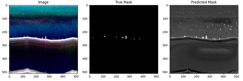
The selected model achieved an average recall of roughly 0.89 for fish pixels and 1.0 for background, meaning that nearly 89 % of annotated fish pixels were detected. The average precision was around 0.488, indicating that roughly half of all predicted fish pixels were correct. The relatively low precision reflects the limited annotation coverage in the dataset – many regions predicted as fish were unlabelled in the training data.

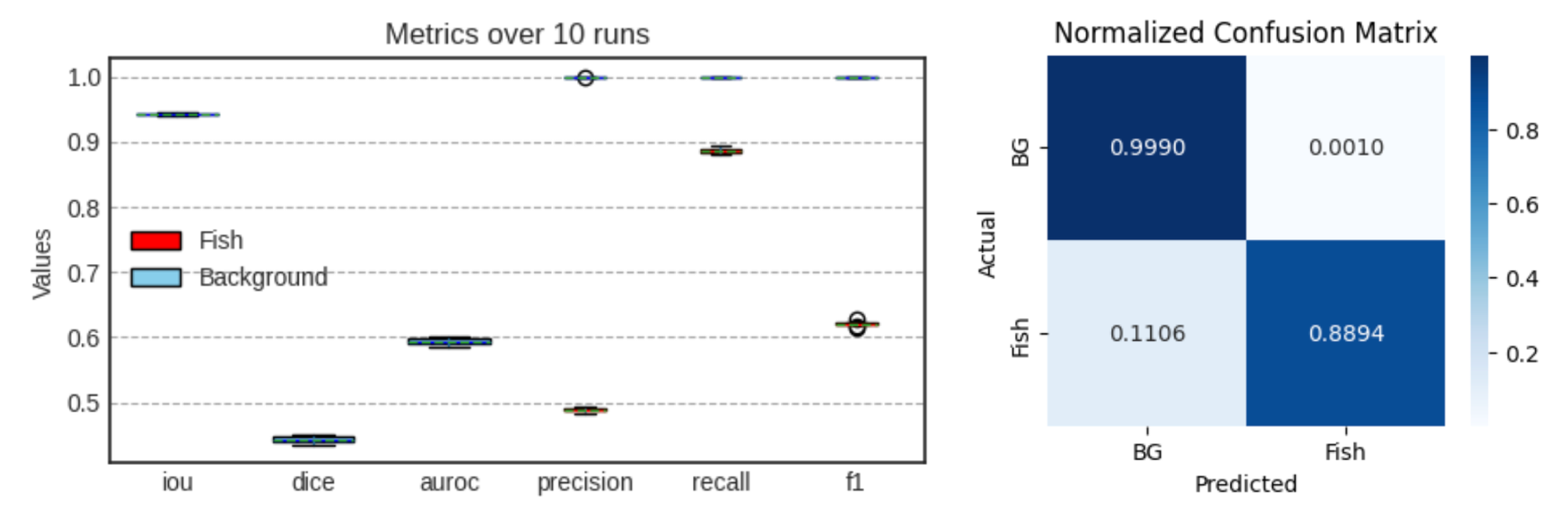
The F1‑score for the fish class averaged 0.62, while the background F1‑score was near perfect. The AUROC averaged 0.943 for both classes, demonstrating strong discrimination between fish and background across probability thresholds. A normalised confusion matrix illustrates that false negatives were primarily due to small clusters being missed, whereas false positives often corresponded to seabed features or noise.

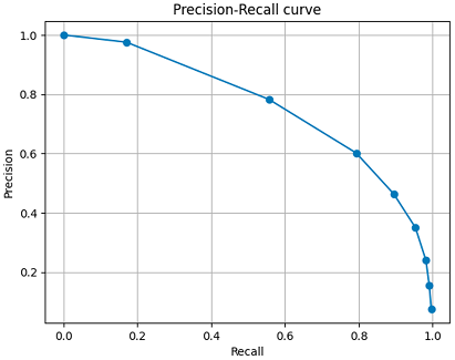
The precision–recall curve highlights how precision declines as recall increases. A threshold of 0.5 yielded the best balance for this dataset.

For a more in-depth tutorial of the training implementation, including the notebook, see our related article:

Training a Deep Learning Model for Echogram Semantic Segmentation

In this tutorial we build a deep‑learning pipeline for echogram segmentation using open‑source tools. Echograms are two‑dimensional plots of acoustic echo intensity versus time and depth recorded using sonar instruments, in our case echosounders.

OceanStreamAndrei Rusu

Training Workflow

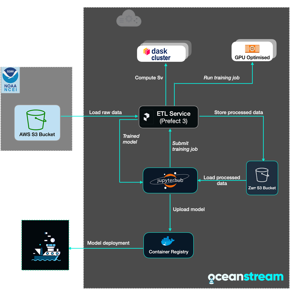
The diagram below shows the entire workflow for training and deployment that we've used for this project and which can be re-used for other similar tasks:

1. EK60 raw data is loaded from the NOAA S3 bucket together with annotations
2. data is processed into images and masks using echopype and echoregions
3. a training job is run on a GPU cluster via the ETL service (Prefect 3)
4. the resulting model is packaged into a container and stored in the container registry
5. the container is deployed to the Edge Box (which is connected to on-board sensors) for local AI inference

Edge‑to‑Cloud Architecture

OceanStream uses the Azure IoT Edge architecture to push computing to the point of data collection while maintaining connectivity to powerful cloud resources. Internet‑of‑Things (IoT) platforms typically focus on collecting sensor readings and streaming them to the cloud for analysis.

In contrast, edge computing refers to executing computational workloads on or near the sensors themselves, thereby reducing the latency and bandwidth required to transmit raw data. 

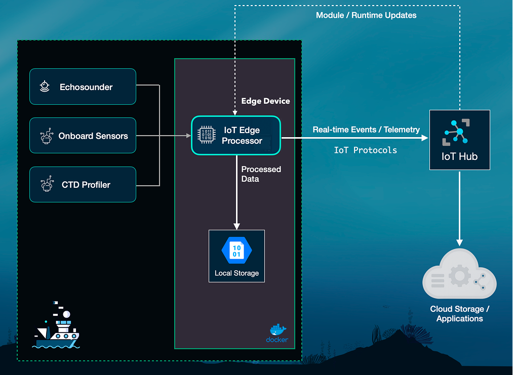
The OceanStream architecture is made of the following components:

• Edge device: Advantech Jetson Orin NX with Ubuntu 22.04 + Docker; runs Azure IoT Edge runtime and OceanStream modules (ingest, Sv compute, ML inference, and buffering to local blob).
• Cloud: Azure IoT Hub, Event routing, Azure Blob/Data Lake for long‑term storage; GPU training clusters orchestrated by Prefect 3 deployments for reproducible runs and on‑demand re‑training.
• Workspaces: Scientific workspaces (JupyterHub) mount Zarr stores for exploratory science, and dashboards render inference overlays for rapid QC.

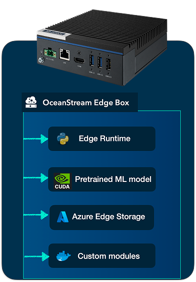
Depending on customer requirements the Edge Box can be supplied in variants featuring the Jetson Orin™ NX or Jetson Nano. The unit is provisioned and configured prior to deployment, allowing the research team to focus on data collection rather than system integration.

Edge compute is invaluable when bandwidth is constrained or when operators need immediate feedback to adjust instrument settings (pulse lengths, ping rates) or survey patterns. 

Generating predictions in real-time

The Edge device is installed on board the ship and is connected to the cloud service via a secure bi‑directional link. The ML detection model is deployed and running on the edge device, packed as a Docker container and can make the predictions on the incoming raw data from the echosounder, in near real-time.

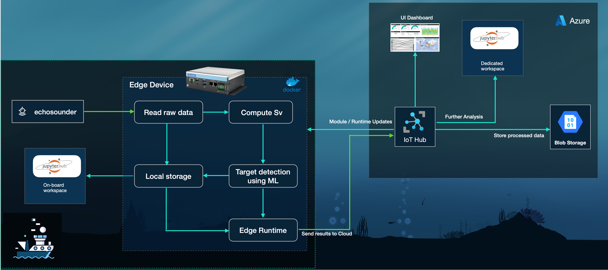
The data flow then will follow the following process:

1. raw data is streamed from the echosounder and auxiliary sensors (such as CTD profilers and GPS) to the IoT Edge processor;
2. the processor computes Sv values from the raw data and then applies the ML models for target detection and segmentation;
3. both the intermediate and final data products are stored locally and can be inspected by on-board staff;
4. when connectivity allows, the device transmits processed summaries and status information to the cloud IoT Hub;
5. cloud endpoints then ingest the processed data into an Azure Blob Storage container as Zarr and populate dashboards, or trigger alerts;
6. the cloud can also deliver module updates and configuration changes back to the vessel, enabling adaptive workflows during surveys.

This distributed pipeline minimises satellite data transmission and thus optimises costs and provides near real‑time situational awareness to staff on shore.

Conclusion and roadmap

The results of this experiment demonstrate the feasibility of using IoT Edge architecture and techniques to assist marine and oceanographic research surveys. Our proposed Edge device, based on NVIDIA Jetson Orin™ NX, is capable of applying deep learning to water column sonar data in near-real-time.

Even with a modest amount of training data, the ML model managed to detect 90% of the pixels the scientists marked as fish schools. The model, however, was a bit too eager, with only about 50% of the pixels it marked actually matching what the experts had identified. We also found cases where the model seemed to catch fish schools that weren't human annotated, showing that the ML model sometimes can spot details experts might overlook.

While these results are promising, this model should still be considered a research prototype rather than production-ready. Its current performance makes it valuable for exploring annotation workflows, benchmarking, and developing new training strategies, but not yet for operational use. We plan to refine the model through additional cross-validation on diverse datasets.

We also plan to explore self‑supervised learning techniques that learn general acoustic features without labels, in order to overcome the limited availability of expert-validated annotations. These pretrained models can then be fine‑tuned on smaller species‑specific datasets. Active learning, where the model suggests the most informative samples for annotation, may also reduce human effort.

We welcome collaborations with researchers and institutions who have Echoview annotation files or other validated segmentation data and are interested in applying or co-developing ML approaches for hydroacoustic analysis.

Authors: Andrei Rusu; Katja Ovchinnikova; Yang Yang